From CCTV to Safer Crosswalk Timing

Traffic signals are often designed around a simplified assumption: pedestrians cross at a standard walking speed. But that assumption is not equally safe for everyone.

In South Korea, elderly pedestrians can walk much slower than the timing used in many standard crossing calculations. The project in rashiedomar/crosswalk-cctv starts from that public-safety problem and turns it into a computer vision system: detect the crosswalk region from overhead CCTV, use that region as the area of interest, and eventually estimate pedestrian crossing speed so signal timing can adapt to slower walkers.

The full research roadmap has four phases:

1. Crosswalk segmentation from CCTV.
2. Pedestrian detection, tracking, and speed estimation.
3. Adaptive timing control and safety validation.
4. Edge deployment on Jetson-style hardware.

This article focuses on Phase 1, which is already complete: building a robust crosswalk segmentation model that transfers from first-person-view data to overhead CCTV. The result is strong: 98.5% IoU on CCTV validation images, using only 241 manually labeled CCTV images plus 1,000 high-confidence pseudo-labels selected from 5,926 unlabeled AI-Hub CCTV images.

That number matters, but the more interesting story is how the project got there.

Why Crosswalk Segmentation Comes First

Adaptive signal timing needs a reliable definition of where crossing happens. Before estimating pedestrian speed, the system must know the crosswalk region:

• where pedestrians enter,
• where they leave,
• which pixels belong to the legal crossing zone,
• and which moving objects should be ignored because they are outside the crosswalk.

If the crosswalk mask is wrong, every downstream step becomes fragile. A pedestrian tracker may detect people, but without a reliable region of interest it cannot tell whether a person is actually crossing, waiting, passing near the curb, or walking on the sidewalk.

So Phase 1 is a segmentation problem:

Given an image $X \in \mathbb{R}^{H \times W \times 3}$, predict a binary mask:

where each pixel $\hat{Y}_{ij}$ estimates whether pixel $(i,j)$ belongs to the crosswalk.

The target mask is:

Once the mask is reliable, the later pedestrian-speed pipeline can restrict analysis to the crosswalk area:

where $\odot$ means element-wise masking.

That sounds simple, but the camera viewpoint changes everything.

The Domain Gap

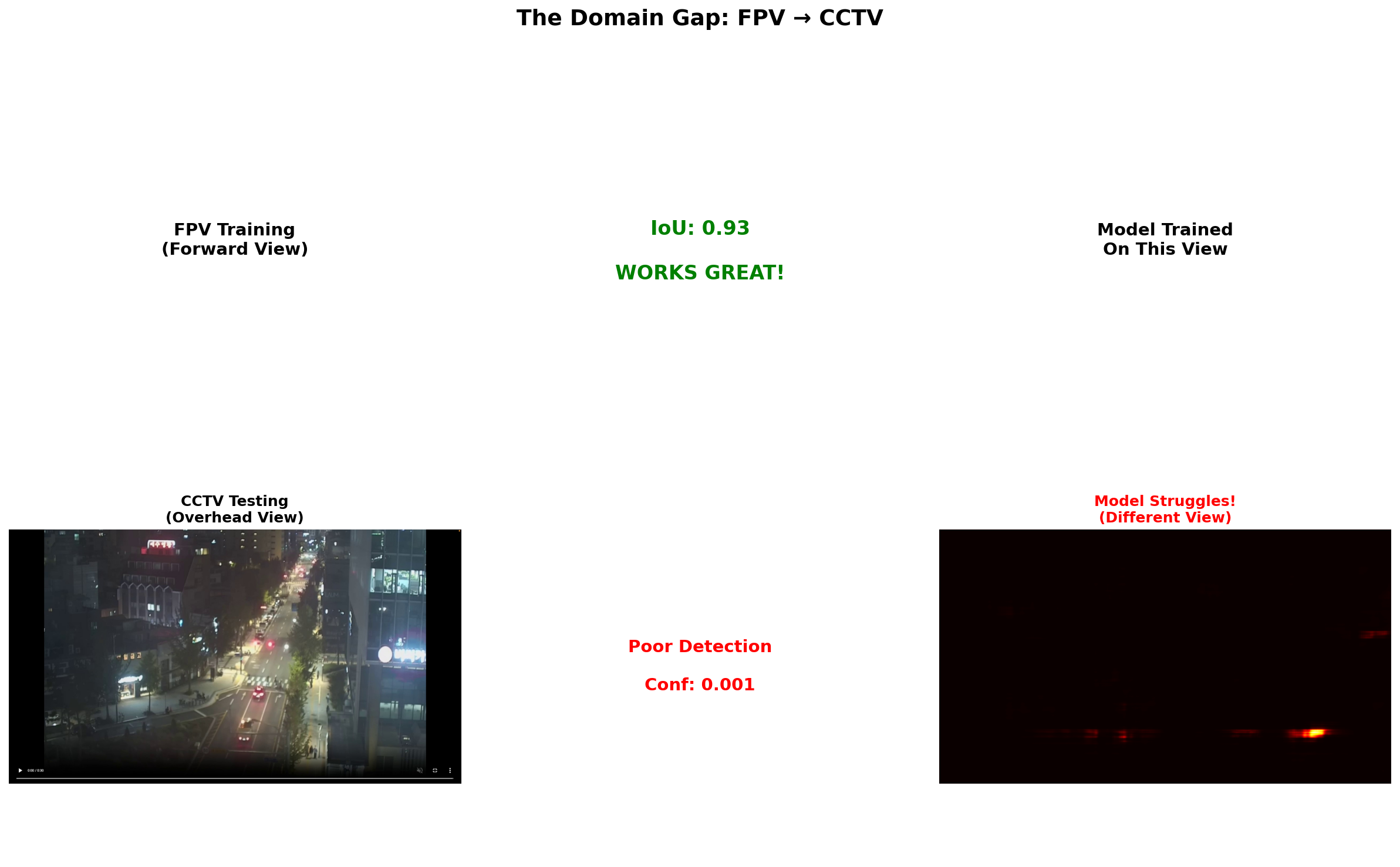
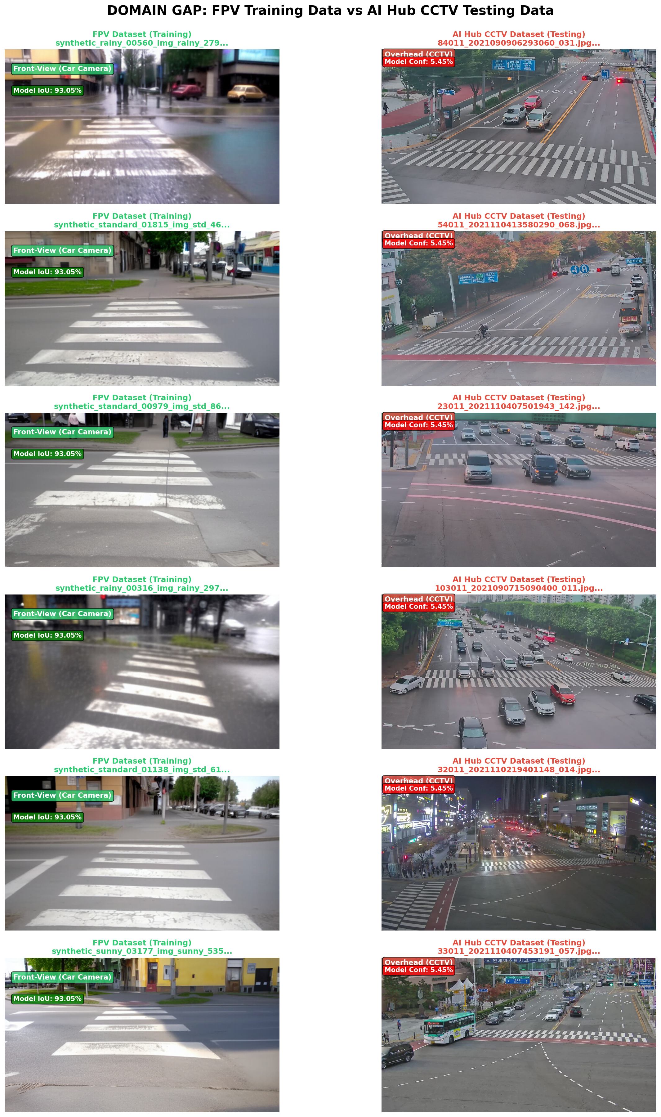
The first model was trained on first-person-view crosswalk images. In that domain, crosswalks are usually seen from a driver or street-level perspective. The stripes are large, close, and often occupy a predictable region of the image.

The target domain is overhead CCTV. In CCTV footage, crosswalks are smaller, farther away, angled, partially occluded by cars or buses, affected by rain or night lighting, and often surrounded by road markings that look similar.

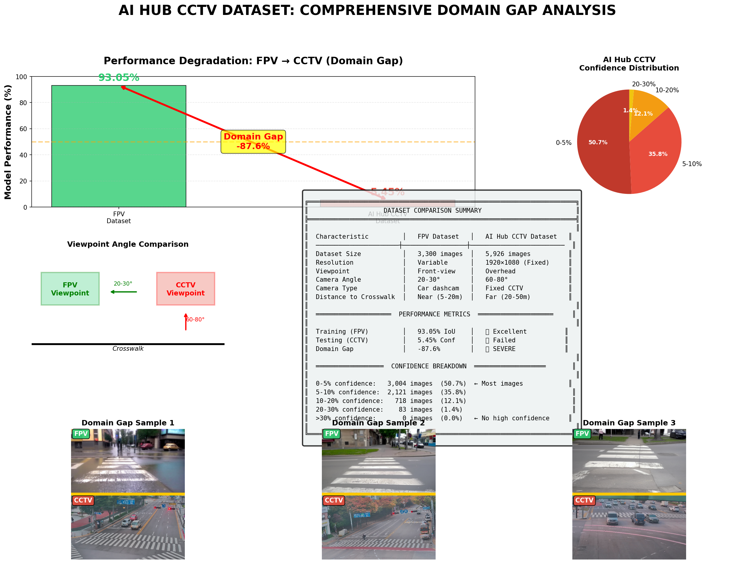
The FPV model performed well on its own domain, reaching about 93.05% IoU on the FPV test set. But when tested directly on CCTV, the confidence collapsed.

This is the classic domain adaptation problem. The model did not only learn “crosswalkness.” It also learned the appearance distribution of the training domain:

In the source domain:

In the target CCTV domain:

The task is the same, but the data distribution changes:

That mismatch is enough to make a high-performing source model fail. The project therefore uses the FPV model as a starting point, not as the final detector.

Stage 1: FPV Baseline

The first stage trained a U-Net model with a ResNet34 encoder on 3,300 FPV crosswalk images. U-Net is a natural starting point because it combines encoder features with decoder upsampling and skip connections.

For segmentation, the model learns a function:

where $\theta$ are the model parameters.

The basic evaluation metric is Intersection over Union:

For binary masks, this can be written as:

where $TP$ is the number of correctly predicted crosswalk pixels, $FP$ is the number of false crosswalk pixels, and $FN$ is the number of missed crosswalk pixels.

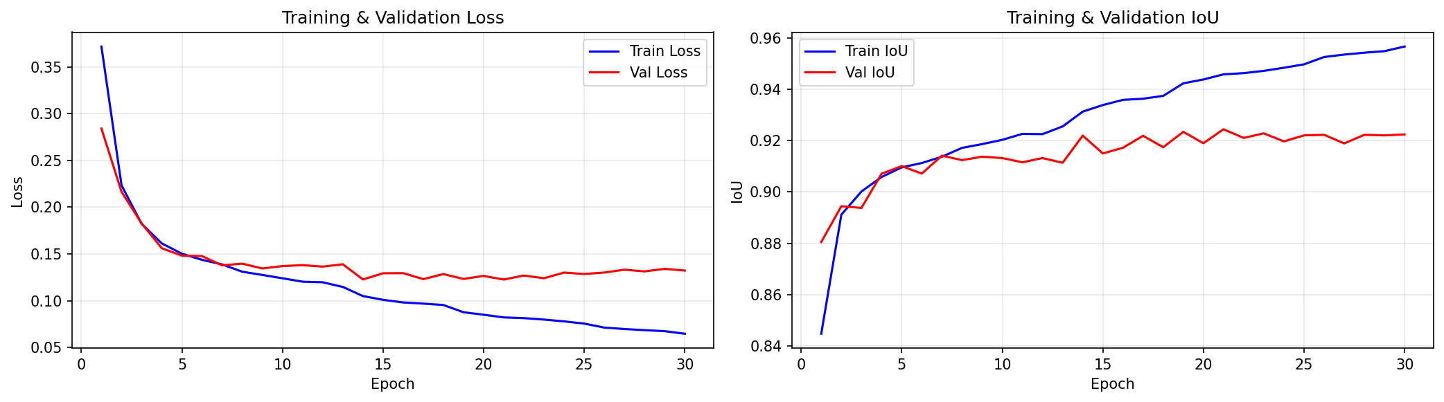
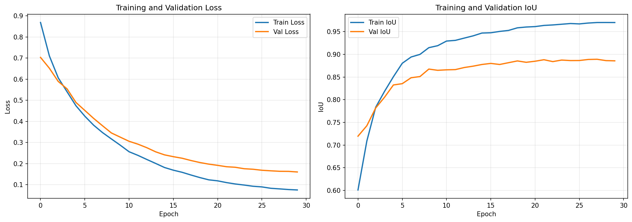
The FPV baseline reached:

• best validation IoU: 92.44%
• test IoU: 93.05%
• training epochs: 30

This is a strong result inside the FPV domain. But it does not solve the CCTV problem. A model can look excellent on a source domain while still being unreliable in the deployment domain.

That is why the next stage matters.

Testing the Source Model on CCTV

When the FPV-trained model was tested on overhead CCTV frames, the model struggled. On one CCTV set of 175 frames, the mean confidence was only about 0.044. Night frames were especially weak, with an average confidence close to 0.0016, while day frames averaged about 0.106.

The AI-Hub CCTV evaluation showed the same pattern. Across 5,926 CCTV images, mean confidence was only about 0.0545, with most images below 10% confidence.

This failure is useful. It proves that the deployment domain needs its own adaptation step.

The lesson is not “the FPV model is bad.” The lesson is that viewpoint matters. A first-person crosswalk and an overhead CCTV crosswalk are visually different objects from the perspective of the model.

The visual comparison makes the problem even clearer. FPV examples tend to show crosswalk stripes as near-field objects with strong perspective expansion. CCTV examples compress the same structure into a distant, oblique region of the frame. The lane markings, bus lanes, reflections, headlights, and road arrows become distractors.

This is one reason crosswalk segmentation is a better first target than pedestrian speed estimation. If the system cannot first localize the crosswalk under viewpoint shift, any attempt to estimate speed inside the scene will mix true crossing motion with irrelevant road and sidewalk motion.

Stage 2: CCTV Adaptation

The second stage adapts the model to CCTV. The key difficulty is annotation cost. Manually labeling CCTV segmentation masks is slow, and the project starts with only 241 labeled CCTV images:

• 201 training samples
• 40 validation samples

The first CCTV adaptation pass fine-tuned a DeepLabV3 model with a ResNet50 backbone. DeepLabV3 is useful here because atrous convolution and multi-scale context help segmentation models capture structure across different receptive fields.

The loss combines binary cross-entropy and Dice-style overlap:

Binary cross-entropy handles pixel-wise classification:

Dice loss focuses on region overlap:

The first CCTV fine-tuning pass reached:

• best validation IoU: 88.9%
• final train IoU: 97.0%
• epochs: 30

That is already usable, but the gap between train and validation suggests a familiar problem: the labeled dataset is small. The model can learn the 241 labeled images, but the target CCTV distribution is wider than those labels.

The project therefore uses semi-supervised learning.

Data Preparation Matters

Before the model can learn anything useful, the project has to convert video and image sources into a consistent segmentation dataset.

That preparation step is not glamorous, but it is where many applied computer vision projects succeed or fail. Crosswalk segmentation needs image-mask pairs that agree spatially. If a frame is resized, cropped, padded, or augmented, the mask must receive the same transformation.

The dataset workflow in the repository is notebook-driven:

• extract frames from video sources,
• prepare FPV training images,
• visualize FPV and CCTV differences,
• train the FPV baseline,
• test the FPV model on CCTV,
• fine-tune and pseudo-label CCTV data.

The important design decision is keeping the experiment stages separate. The project does not hide everything inside one giant script. It preserves the story of the research:

1. Build a source-domain baseline.
2. Measure how badly it transfers.
3. Add limited labeled target data.
4. Use target-domain unlabeled data.
5. compare iteration 1 and iteration 2.

That structure makes the result easier to trust. If someone only reports the final 98.5% IoU, we do not know how much was learned from source data, how much came from manual labels, and how much came from pseudo-labels. Here, each stage has its own artifacts.

Architecture Choice

The final adaptation uses DeepLabV3 with a ResNet50 backbone. That is a reasonable choice for CCTV crosswalk segmentation because the object has both local and global structure.

The local structure is the stripe pattern. A model must identify repeated white bars, edges, and road-paint texture.

The global structure is the crosswalk polygon. A crosswalk is not just a set of stripes; it is a coherent region across the road. It has orientation, width, continuity, and geometric plausibility.

DeepLab-style models help because they can combine fine visual cues with broader context. In practice, the model needs to answer questions like:

• Are these stripes part of a legal crosswalk or just lane markings?
• Does the predicted region form a plausible crossing zone?
• Does the mask remain stable under shadows, vehicles, and camera angle?
• Can the model see the full crosswalk even when part of it is occluded?

For this phase, a binary segmentation model is the right abstraction. The output is not a bounding box, because a crosswalk is not always rectangular in image coordinates. The output is not a classification label, because the exact region matters for later speed estimation. A dense mask is the useful representation.

Pseudo-Labeling

Pseudo-labeling is the bridge between scarce manual labels and abundant unlabeled data.

Let the labeled set be:

and the unlabeled set be:

After training an initial model $f_{\theta_1}$ on $\mathcal{D}_L$, we generate predicted masks for the unlabeled images:

But we should not trust every prediction. The project filters pseudo-labels using a confidence score and geometric validation.

The idea is:

where:

• $c_j$ is prediction confidence,
• $g_j$ is geometric validity,
• and $q_j$ is the final pseudo-label quality score.

The geometric check is important because crosswalk masks have physical structure. They should not occupy almost none of the frame, and they should not cover almost the whole frame. The project uses a reasonable crosswalk-area constraint, roughly checking whether the predicted mask occupies a plausible percentage of the image.

In simplified form:

The repository describes the accepted area ratio range as about 5% to 40% of the frame.

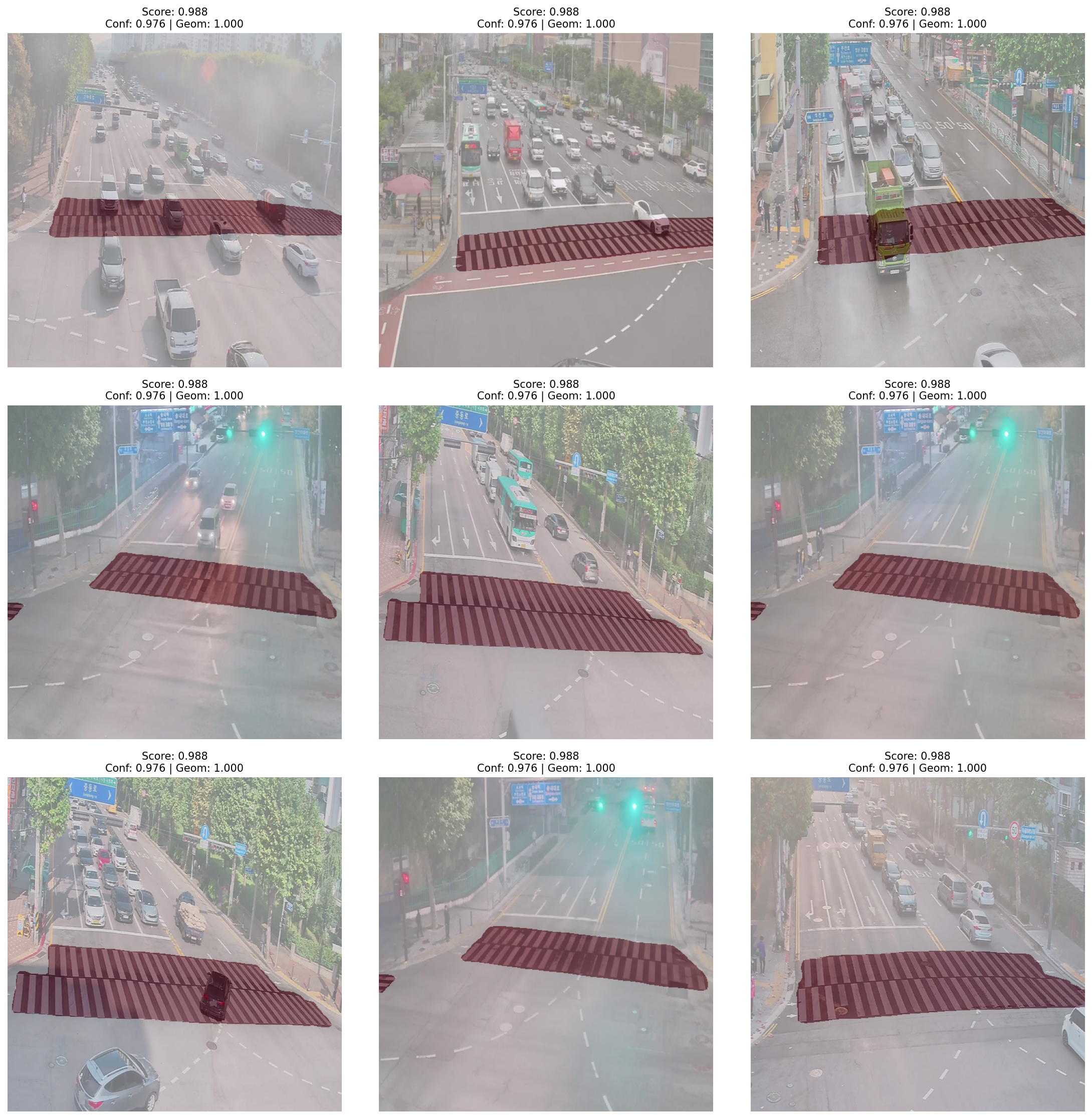
From 5,926 unlabeled CCTV images, the system selected the top 1,000 high-confidence pseudo-labels using a threshold of 0.7. The top pseudo-label scores were extremely high:

• top score: 0.988
• median score: 0.988
• confidence score around 0.976
• geometric validation: 1.0 for the top samples

This step increases the effective training set from 241 CCTV images to 1,241 images:

The key is not just adding more data. It is adding more target-domain data: new lighting, roads, camera angles, vehicles, road widths, shadows, and crosswalk geometries.

Why Confidence Alone Is Not Enough

One nice detail in this project is that pseudo-label selection is not based on raw model confidence alone.

Raw confidence can be misleading. A segmentation model can be confidently wrong, especially after domain shift. It may draw a large mask over a road area, produce a tiny blob near a bright lane marking, or hallucinate a crosswalk where none exists. If we accept those masks because the probabilities are high, pseudo-labeling becomes error amplification.

That is why geometric validation matters. Crosswalks have expected shape and scale. They usually occupy a meaningful but limited part of the frame. They are often elongated and road-aligned. A simple geometry rule will not solve all errors, but it can reject many obviously bad pseudo-labels.

This gives the pseudo-labeling step two checks:

1. Does the model believe the mask?
2. Does the mask look physically plausible?

That is a strong pattern for applied AI. Confidence should be combined with domain knowledge whenever possible.

Iteration 2: Training with Pseudo-Labels

The second iteration retrains on the combined dataset:

• 241 manually labeled CCTV images
• 1,000 pseudo-labeled CCTV images
• 1,241 total target-domain examples

The learning rate is reduced to stabilize adaptation. The model has already learned the rough CCTV crosswalk concept, so the next stage is refinement and generalization.

The result is the main achievement of Phase 1:

• Iteration 1 validation IoU: 88.9%
• Iteration 2 validation IoU: 98.5%
• improvement: +9.6 percentage points
• inference time: 12.98 ms
• throughput: 77.03 FPS

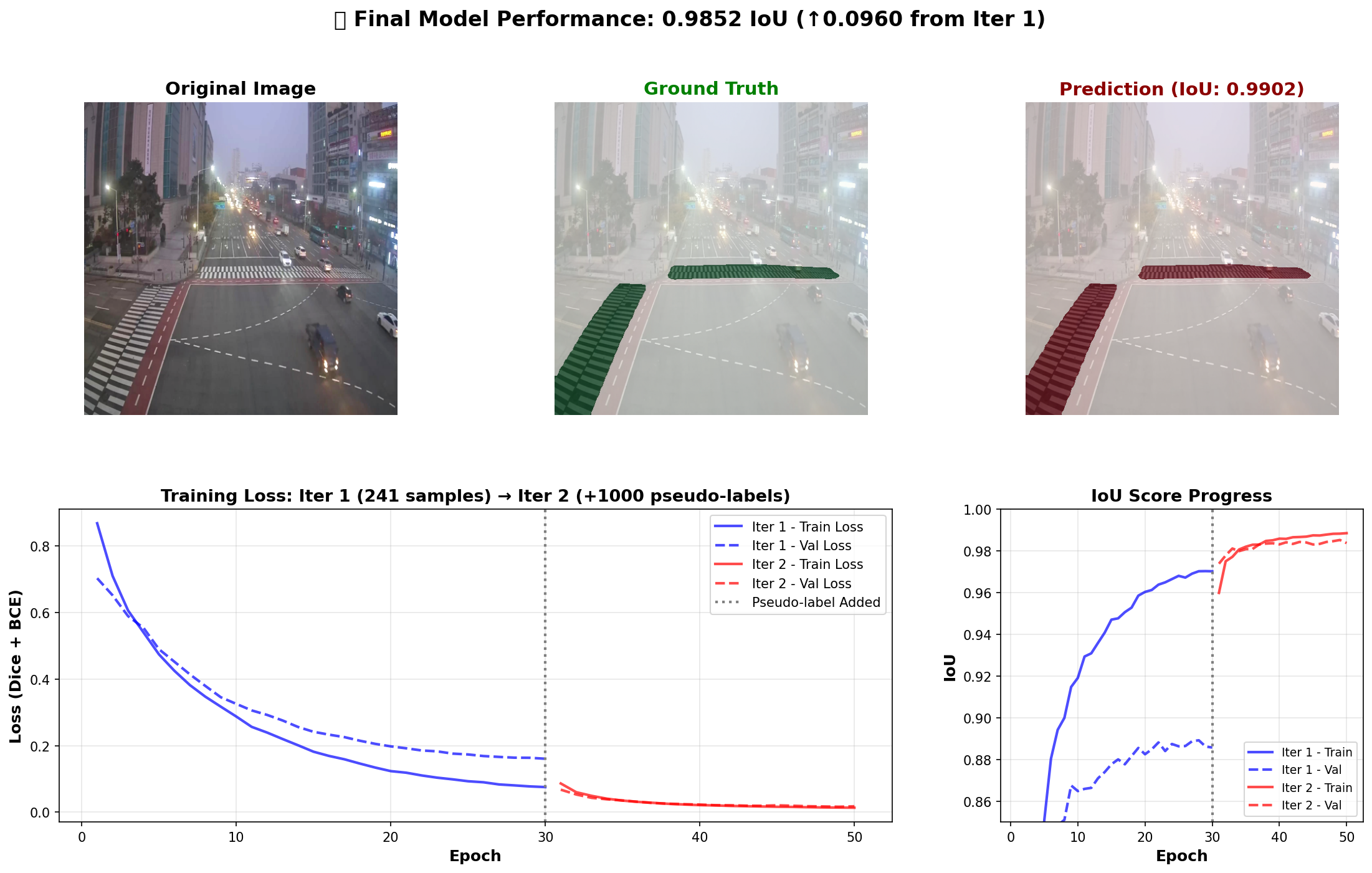
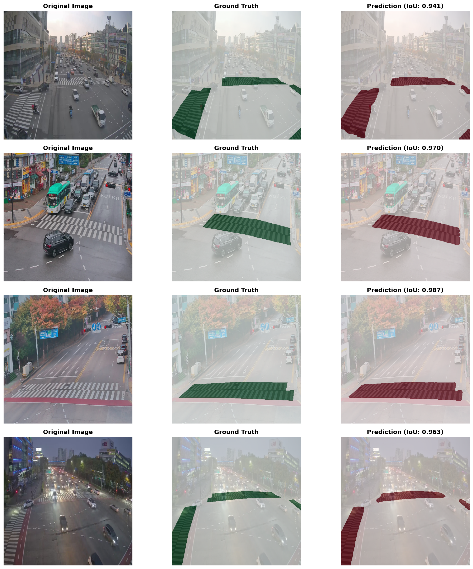
The final visualization shows why the result is convincing. The predicted mask aligns closely with the manual ground-truth crosswalk region, even under overhead perspective and real CCTV conditions.

This is exactly what a Phase 1 module should provide: a stable, fast crosswalk mask that later components can use as the spatial foundation for pedestrian tracking.

Reading the Result Carefully

The final result figure is impressive, but it is worth reading it like a researcher instead of only like a scoreboard.

The top row shows an original CCTV image, a manual ground-truth mask, and a model prediction. The prediction nearly overlaps the target crosswalk region, and the figure reports an IoU around 0.99 for that example.

The bottom plots tell the training story. Iteration 1 improves quickly but plateaus below the final result. After pseudo-labeling is added, iteration 2 starts from a much stronger place and pushes validation IoU close to the training IoU. This means the additional target-domain data did not only help the model memorize. It helped it generalize better across the validation samples.

The result is also practical because the prediction is spatially clean. A noisy mask with many disconnected blobs would be hard to use for tracking. A clean crosswalk polygon can be post-processed into a stable region of interest.

Why the Result Works

The performance jump is not magic. It comes from three design choices working together.

First, transfer learning gives the model a useful starting point. The FPV source task still teaches stripes, road texture, crosswalk shape, and segmentation boundaries. Even if the viewpoint is wrong, the learned representation is better than random initialization.

Second, small labeled CCTV fine-tuning anchors the model to the target viewpoint. The 241 manual masks teach the overhead camera geometry.

Third, pseudo-labeling expands the target domain. The extra 1,000 pseudo-labels expose the model to many more CCTV conditions without requiring full manual annotation.

The training process can be summarized as:

for the source FPV model, then:

for the first CCTV adaptation, and finally:

where $\mathcal{D}_P$ is the pseudo-labeled set and $w(u)$ can be interpreted as a confidence weight. Even when the implementation uses selected pseudo-labels rather than explicit continuous weights, the idea is the same: high-confidence pseudo-labels are allowed to influence training.

This is data-efficient domain adaptation.

Real-Time Requirement

A research model is not enough for an adaptive signal system. The system must run fast enough to support live CCTV.

At 512 by 512 resolution, the final model runs at about 77 FPS, corresponding to roughly 12.98 ms per frame. That exceeds a 30 FPS real-time target:

With $t_{\text{ms}} = 12.98$:

That speed matters because Phase 2 will add more computation: pedestrian detection, tracking, trajectory smoothing, and speed estimation. If segmentation already consumes the full time budget, the later system will fail. A fast segmentation module leaves room for the rest of the pipeline.

In deployment terms, this means the segmentation model can run as a front-end perception module. It does not need to recompute a brand-new crosswalk mask at every frame if the camera is fixed. A practical system could compute or update the mask periodically, stabilize it across time, and then use it as a fixed region for tracking. That would save compute for pedestrian detection and trajectory estimation.

For fixed CCTV, the crosswalk itself is mostly static. The hard part is not that the crosswalk moves; it is that lighting, shadows, weather, vehicles, and occlusions change. So the segmentation module can be used in two ways:

• as a one-time or periodic crosswalk locator,
• and as a robustness check when the scene changes significantly.

This is important for edge deployment. On a Jetson-like device, every millisecond matters.

Toward Speed Estimation

Once the crosswalk mask is stable, Phase 2 can estimate walking speed.

For a tracked pedestrian, suppose their position in image coordinates at time $t$ is:

A tracker such as DeepSORT can maintain an identity across frames:

To estimate physical speed, image movement must be converted into meters. With a calibration function $H$ or a pixel-to-meter scale, positions can be projected into ground-plane coordinates:

Then walking speed can be estimated as:

The signal timing problem is then straightforward. If the crosswalk length is $L$ and a pedestrian walks at speed $v$, the required crossing time is:

The safety issue appears when the assumed design speed is too high:

If $v_{\text{elderly}} < v_{\text{standard}}$, then:

That is the entire motivation of the project in one equation. Slower pedestrians need more crossing time. A vision system can estimate when that extra time is needed.

The next research challenge is not only measuring speed, but measuring it reliably. A pedestrian may pause, turn, walk diagonally, start late, or be occluded by a vehicle. A simple two-point speed estimate can be noisy. A stronger version would estimate speed over a track:

Then the system can smooth speed over time:

This kind of smoothing prevents one noisy frame from causing unstable signal decisions.

What Makes This Project Strong

The strongest part of this project is that it does not jump directly to signal control. It builds the perception foundation first.

A weaker version of the project would try to detect pedestrians everywhere in the frame and estimate speed immediately. But without a crosswalk mask, the system would have too much ambiguity. People on sidewalks, people waiting near the curb, cyclists, reflections, and vehicles could all interfere with the logic.

This project begins with the spatial prior:

Where is the crosswalk?

Once that is known, later modules can ask better questions:

• Is a person inside the crosswalk?
• How long have they been crossing?
• Are they moving slower than expected?
• Are they likely to remain in the crosswalk when the signal changes?
• How much extra green time is needed?

This is good system design. Perception, tracking, speed estimation, and control are separated into stages.

Limitations

The Phase 1 result is strong, but it should be interpreted carefully.

First, the final model is evaluated on the available CCTV validation set. More cities, weather conditions, camera heights, road geometries, and nighttime scenes would be needed before claiming broad deployment readiness.

Second, pseudo-labeling works best when the first model is already good enough. If the first fine-tuned model produces systematically wrong masks, pseudo-labeling can amplify errors.

Third, segmentation accuracy does not guarantee tracking accuracy. Phase 2 still needs robust pedestrian detection and identity tracking under occlusion, crowding, shadows, vehicles, and low-light conditions.

Fourth, signal timing is a control problem, not only a vision problem. It must consider traffic rules, pedestrian signals, vehicle flow, fairness, and safety margins.

These limitations do not weaken the project. They define the next research steps.

What I Would Improve Next

If I were extending this project, I would keep the staged design and add a few evaluation layers.

First, I would create a held-out CCTV benchmark split by condition: day, night, rain, heavy traffic, low traffic, bus occlusion, wide intersection, narrow intersection, and unusual camera angle. A single validation number is useful, but condition-specific metrics tell us where the model is fragile.

Second, I would add temporal stability metrics. Since CCTV is video, the mask should not flicker frame by frame. Even if per-frame IoU is high, unstable edges can hurt downstream tracking. A simple temporal consistency score could compare consecutive predictions:

High temporal consistency would mean the crosswalk region remains stable unless the scene truly changes.

Third, I would add uncertainty maps. If the model is uncertain near the boundary or under occlusion, later stages should know that. A tracker can behave differently when the crosswalk ROI is high-confidence versus partially uncertain.

Fourth, I would connect the segmentation output to a small tracking prototype. Even a simple YOLO + DeepSORT baseline inside the predicted ROI would validate that Phase 1 provides the right representation for Phase 2.

Fifth, I would document failure cases as carefully as successes. The best projects show where the model breaks. Night reflections, bus occlusion, unusual crosswalk paint, construction zones, and wet roads are not edge cases for deployment; they are normal urban conditions.

Lessons

There are a few lessons I would take from this work.

The first lesson is that domain shift is real. A model that works in FPV does not automatically work in CCTV.

The second lesson is that small labeled datasets can still be powerful if used strategically. The 241 CCTV labels were enough to bootstrap a useful target-domain model.

The third lesson is that pseudo-labeling is most useful when filtered. The important contribution is not generating 5,926 masks. It is selecting the 1,000 masks that are confident and geometrically plausible.

The fourth lesson is that real-time performance should be measured early. A safety system cannot wait until the end to discover that it is too slow.

Conclusion

The crosswalk CCTV project is a strong example of applied computer vision research because it connects model design to a real public-safety workflow.

The system starts with a concrete social problem: elderly pedestrians may need more crossing time than standard signal assumptions provide. It then builds a technical foundation: crosswalk segmentation from CCTV. It handles the domain gap from FPV to overhead camera views, uses a small manually labeled CCTV set, expands it with confidence-filtered pseudo-labels, and reaches 98.5% IoU at 77 FPS.

That makes Phase 1 ready to support the next stage: pedestrian tracking and speed estimation inside the detected crosswalk region.

You can read the code, inspect the notebooks, and fork the project here:

GitHub: rashiedomar/crosswalk-cctv